Understanding Fairness Notions in Data-Driven Decision Making#
In data-driven decision making, algorithmic systems can encode and amplify bias. We see the reflection of societal biases in training datasets, and in development assumptions [Jacobs and Wallach, 2021]. Indeed, researchers and practitioners actually encode bias while constructing “measurement models” to quantify abstract concepts as a combination of observed features. This process is referred as measurement modeling can introduce potential mismatches between the theoretical understanding and its operationalization [Jacobs and Wallach, 2021]. Jacobs et al. argues that fairness-related harms are mainly a result of such mismatches.
In this notebook, we explain common fairness notions and possible metrics to fulfil this notion. A fairness notion refers to the conceptual idea or principle behind what it means for a system to be fair, such as “equal treatment” or “equal outcomes.” A fairness metric, on the other hand, is a specific, measurable way to evaluate whether a system adheres to a particular fairness notion, often using statistical methods.
The fairness notions can be broadly categorized into group fairness and individual fairness, each addressing different dimensions of fairness. Group fairness, also known as “statistical fairness”, focuses on treating different social groups equally. Individual fairness advocates for similar treatment for similar individuals.
Group Fairness#
The key objective of group fairness is satisfying the independence by ensuring sensitive characteristics are independent of the prediction results. It seeks to provide statistically fair guarantees for groups defined by sensitive attributes like race or education level. These fairness notions aim to prevent biases against specific groups, promoting equal treatment in decision-making processes. Four commonly used group fairness notions are:
Demographic parity [Zemel et al., 2013] (Related metrics: Positive Rate / Negative Rate) demands equal prediction rates across groups defined by sensitive attributes such as race or gender. It ensures that individuals from different social groups receive equal treatment in the decision-making process, regardless of their background.
In a binary classification problem, where each sample point is represented by a given feature set X, binary sensitive feature A, true outcome Y, and predictions $\(\hat{Y}\)$, we can define statistical parity formally as:
\[ Pr(\hat{Y} | A = 0) = Pr(\hat{Y} | A = 1) \]We will use the same notations for the rest of this article.
Equalised odds [Hardt et al., 2016] (Related metrics: True Negative Rate / False Negative Rate or True Positive Rate / False Positive Rate) depend on the target value (Y) as a form of ground truth about the classification’s accuracy.
\[ Pr(\hat{Y} = 1| A = 0, Y = y) = Pr(\hat{Y} = 1| A = 1, Y = y) \]Equal opportunity [Hardt et al., 2016] (Related metrics: True Positive Rate / False Negative Rate or True Negative Rate / False Positive Rate) is another group fairness metric, focuses on ensuring that individuals from different demographic groups have an equal chance of positive outcomes (true positives), such as being hired for a job or receiving a loan.
\[ Pr(\hat{Y} = 1|Y = 1, A = 0) = Pr(\hat{Y} = 1|Y = 1, A = 1) \]Calibration (Related metrics: False Discovery Rate, False Omission Rate) is a key aspect of group fairness, focuses on ensuring that the predicted probabilities align with the true probabilities of positive outcomes for different demographic groups. Calibration within groups means having equal true positive probability for the same predicted score ((S=s)) irrespective of the sensitive feature [Kleinberg et al., 2016].
\[ Pr(Y = 1|S = s, A = 0) = Pr(Y = 1|S = s, A = 1) \quad \forall s \in [0, 1] \]
Individual Fairness#
Individual fairness can be seen as fine-grained fairness by demanding comparable predictions for individuals with similar characteristics. The motivation behind individual fairness is to avoid favouring less qualified individuals over more qualified ones. Examples of individual fairness notions include causal discrimination, fairness through awareness, counterfactual fairness, and no unresolved discrimination. These notions strive to ensure fairness at an individual level, promoting equal opportunities for all individuals regardless of their background.
Fairness through awareness is a distance-based metric to measure the distance of probability distributions of two individuals over outcomes gives similar results for the individuals with different protected attributes [Dwork et al., 2012].
\[ Dist(Pr(X_i), Pr(X_j)) \leq d(x, y) where d(x, y) denotes the max distance for all individual pairs (x, y) \]This equation represents a fairness criterion where the distance between the probability distributions \(Pr(X_i)\) and \(Pr(X_j)\) is less than or equal to the similarity distance between the individuals \(X_i\) and \(X_j\). It reflects the idea that the difference in predictions should not exceed the similarity between the individuals, ensuring fairness in the decision-making process.
Causal discrimination demands that individuals with similar characteristics or qualifications receive comparable treatment in decision-making processes [Galhotra et al., 2017]. For example, an algorithm is fair with respect to “sensitive attributes” if for all pairs of individuals with the same features other than these sensitive attributes.
\[ Pr(\hat{Y} = 1 | \text{similar}(X_i, X_j)) = Pr(\hat{Y} = 1 | \text{similar}(X_i, X_j), A = 0) \]Counterfactual fairness aims to ensure that individuals would receive the same outcome regardless of their sensitive attributes, had their attributes been different. It considers counterfactual scenarios where individuals’ attributes are changed while keeping other factors constant.
\[ Pr(\hat{Y}(i, d) = y | A = a) = Pr(\hat{Y}(j, d) = y | A = a) \]Where:
\(\hat{Y}(i, d)\) represents the predicted outcome for individual \(i\) under counterfactual scenario \(d\).
\(y\) denotes the predicted outcome.
\(A\) denotes the sensitive attribute.
\(a\) denotes the value of the sensitive attribute.
\(i\) and \(j\) represent individuals.
\(d\) represents the counterfactual scenario.
The technical implementation of fairness notions varies and can target different stages of the decision-making process. This includes correcting input data, exploring feasible solution spaces, representing features graphically, or leveraging fair representation learning techniques. However, combining multiple fairness notions can present challenges, such as inadvertently treating individuals unfairly despite satisfying group fairness or facing mathematical limitations in simultaneously satisfying multiple fairness criteria.
Addressing fairness technically has raised concerns about the trade-offs between accuracy and fairness. While efforts have been made to optimize both, there remains a need to ensure fairness from a societal perspective. This entails aligning the metrics used to measure fairness with societal values and operationalizing fairness in a way that reflects real-world equity concerns.
In conclusion, understanding and implementing fairness notions in data-driven decision-making processes is essential for promoting equity and mitigating biases. By incorporating both group and individual fairness considerations, alongside addressing implementation challenges, we can strive towards more just and equitable outcomes in algorithmic decision making. The figure below summarises the overall relationship between fairness notions and metrics as an ontology diagram:
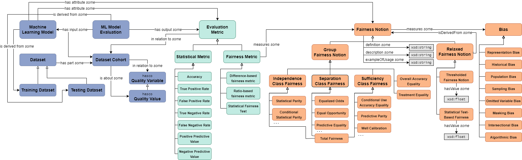 The figure is obtained from [Franklin et al., 2022] and is available on Github.
Useful Resources#
Tensorflow’s Fairness Guidance (https://www.tensorflow.org/responsible_ai/fairness_indicators/guide/guidance) has some practical information on using different notions for different applications.
Fair ML Book to deep dive into the concepts discussed in this article https://fairmlbook.org/classification.html and https://fairlearn.org/v0.7.0/user_guide/fairness_in_machine_learning.html
Also Varshney’s book: http://www.trustworthymachinelearning.com/
Visit this course materials: alan-turing-institute/bias-in-AI-course